


Introduction
This post will demonstrate how to use machine learning to forecast time series data. The data set is from a recent Kaggle competition to predict retail sales.
You will learn how to:
- Build a machine learning model to forecast time series data (data cleansing, feature engineering and modeling)
- Perform feature engineering to build categorical and continuous temporal features
- Identify and plot feature importance
- Utilize a recursive prediction technique for long-term time series forecasting
Time Series Forecasting
Time series forecasting using machine learning is more complex than standard machine learning because the temporal component of the data adds an extra dimension to the problem. Time series forecasting is used across almost all industries. A few examples are:
- Retail Product Sales
- Stock Price Movement
- Agricultural Yields
- Utilization of Resources
- Service Queues
Time series forecasts can be either short-term (e.g. predict tomorrow’s sales) or long-term (e.g. predict sales for the next month). Long-term predictions are more complex because uncertainty increases with the length of the predictive period. The problem we analyze in this post requires long-term predictions. We will use a recursive, multi-step prediction technique which we will discuss in greater detail later in the post.
Data Overview
Competition Description: Corporación Favorita, a large Ecuadorian-based grocery retailer that operates hundreds of supermarkets, with over 200,000 different products on their shelves, has challenged the Kaggle community to build a model that more accurately forecasts product sales.
Dataset: Corporacion Favorita provided historical sales data from 2012 – August 15th, 2017.
Challenge: The challenge is to predict sales from August 16th – August 31st 2017 for a given product at a given store.
Load packages
library(data.table)
library(dplyr)
library(padr)
library(xgboost)
library(Matrix)
library(RcppRoll)
library(zoo)
library(knitr)
library(xtable)
Data Exploration
To speed up the analysis, we will use data from four stores from the dates 2017-07-15 to 2017-08-15, and a subset of the available features.
At the start of any data science problem, it is important to explore the available data. The head(), str() and summary() functions are great for getting a high-level view of the data.
Read and subset test and training data.
train <- fread('https://github.com/MattBrown88/Time-Series-Machine-Learning/raw/master/train_subset.csv')
train$date <- as.character(train$date)

MinDate <- '2017-07-15'
MaxDate <- '2017-08-15'

test <- fread('https://github.com/MattBrown88/Time-Series-Machine-Learning/raw/master/test_subset.csv')
View the first few rows of the data set.
head(train)
##           id       date store_nbr item_nbr unit_sales onpromotion
## 1: 122137474 2017-07-15         1    99197          2       FALSE
## 2: 122137475 2017-07-15         1   103520          1       FALSE
## 3: 122137476 2017-07-15         1   105574          6       FALSE
## 4: 122137477 2017-07-15         1   105575         10       FALSE
## 5: 122137478 2017-07-15         1   105737          3       FALSE
## 6: 122137479 2017-07-15         1   105857          7       FALSE
With these few columns we will be able to create many new temporal features for the model.
View the structure of the data set.
str(train)
## Classes 'data.table' and 'data.frame':   279106 obs. of  6 variables:
##  $ id         : int  122137474 122137475 122137476 122137477 122137478 122137479 122137480 122137481 122137482 122137483 ...
##  $ date       : chr  "2017-07-15" "2017-07-15" "2017-07-15" "2017-07-15" ...
##  $ store_nbr  : int  1 1 1 1 1 1 1 1 1 1 ...
##  $ item_nbr   : int  99197 103520 105574 105575 105737 105857 106716 108696 108698 108797 ...
##  $ unit_sales : num  2 1 6 10 3 7 1 1 4 1 ...
##  $ onpromotion: logi  FALSE FALSE FALSE FALSE FALSE FALSE ...
##  - attr(*, ".internal.selfref")=<externalptr>
View a summary of the target feature (the feature we will be predicting).
summary(train$unit_sales)
##     Min.  1st Qu.   Median     Mean  3rd Qu.     Max.
##  -29.000    2.000    4.000    8.471    8.000 2203.000
The summary of unit_sales shows there are days with negative sales. Below we calculate there are only 24 days with negative unit_sales in the subset of data we chose. This is rare enough that we will just remove these days.
length(train$unit_sales[train$unit_sales < 0])
## [1] 24
train$unit_sales[train$unit_sales < 0] <- 0
Data Cleansing
The evaluation metric of the competition is LRMSE (Log Root Mean Squared Error). The reason for using this metric is to scale the impact of inaccurate predictions. Using the log penalizes predicting 1 when the actual is 6 more than predicting 40 when the actual is 45. We convert unit_sales to log unit_sales here.
train$unit_sales <- log1p(train$unit_sales)
In this problem, the training and test data sets were not in the same format. In the test data set there were entries for items which had zero unit_sales at a given store for a given day. The training data set only contained items on days in which there were unit_sales (i.e. there are no zero unit_sales entries). The training data set needs to include entries for items that were available at a given store on a given day but did not record any unit_sales.
To demonstrate the missing entries from the training data set, here is an example of the original data set subset for a single store and item. Notice how there are no unit_sales from 2017-08-05 to 2017-08-07. We will create new rows for these missing entries and add zero for unit_sales using the padr package.
train_example <- train[train$store_nbr == 1 & train$item_nbr == 103520 & train$date > '2017-08-01',]
train_example[,c('date', 'unit_sales', 'store_nbr', 'item_nbr')]
##          date unit_sales store_nbr item_nbr
## 1: 2017-08-02  0.6931472         1   103520
## 2: 2017-08-03  1.0986123         1   103520
## 3: 2017-08-04  1.3862944         1   103520
## 4: 2017-08-08  1.3862944         1   103520
## 5: 2017-08-10  1.3862944         1   103520
## 6: 2017-08-11  0.6931472         1   103520
## 7: 2017-08-12  0.6931472         1   103520
## 8: 2017-08-13  0.6931472         1   103520
Padr requires the data set have a Date data type field so we convert train$date . The start_val and end_val specify the range from which to add zeros grouped by store_nbr and item_nbr. We only want to add zeros for the range of dates we selected to build the model.
train$date <- as.Date(train$date)

train <- pad(train, start_val = as.Date(MinDate)
             , end_val = as.Date(MaxDate), interval = 'day'
             , group = c('store_nbr', 'item_nbr'), break_above = 100000000000
) %>%
  fill_by_value(unit_sales)
The updated data set is shown below. Notice the new zero unit_sales rows added to the data set.
train_updated <- train[train$store_nbr == 1 & train$item_nbr == 103520 & train$date > '2017-08-01',]
train_updated[,c('date', 'unit_sales', 'store_nbr', 'item_nbr')]
##           date unit_sales store_nbr item_nbr
##  1: 2017-08-02  0.6931472         1   103520
##  2: 2017-08-03  1.0986123         1   103520
##  3: 2017-08-04  1.3862944         1   103520
##  4: 2017-08-05  0.0000000         1   103520
##  5: 2017-08-06  0.0000000         1   103520
##  6: 2017-08-07  0.0000000         1   103520
##  7: 2017-08-08  1.3862944         1   103520
##  8: 2017-08-09  0.0000000         1   103520
##  9: 2017-08-10  1.3862944         1   103520
## 10: 2017-08-11  0.6931472         1   103520
## 11: 2017-08-12  0.6931472         1   103520
## 12: 2017-08-13  0.6931472         1   103520
## 13: 2017-08-14  0.0000000         1   103520
## 14: 2017-08-15  0.0000000         1   103520
The training data set now matches the format of the test data set which is necessary for any chance at an accurate model.
Next, we combine the test and training data sets since we will perform some of the same feature engineering steps on each. We do not want to duplicate code since any extra steps increase the likelihood of mistakes. The fill argument is required because the test and training data sets donât have the same columns; it will fill the test portion of unit_sales with NAs.
train$date <- as.character(train$date)
df <- rbind(train, test, fill = TRUE)
Feature Engineering
Machine learning models cannot simply “understand” temporal data so we much explicitly create time-based features. Here we create the temporal features day of week, calendar date, month and year from the date field using the substr function. These new features can be helpful in identifying cyclical sales patterns.
We convert all of these features to numeric because that is the format required for the machine learning algorithm we will use.
df$month <- as.numeric(substr(df$date, 6, 7))
df$day <- as.numeric(as.factor(weekdays(as.Date(df$date))))
df$day_num <- as.numeric(substr(df$date, 9, 10))
df$year <- substr(df$date, 1, 4)
We separate the training set from the test set now that we have completed the feature engineering which we will do to both.
train <- subset(df, date < '2017-08-16')
Now we will create lag and sliding window variables using the RcppRoll package. These features are the heart of the model and will have the most influence on it’s accuracy. We cannot yet create these features for the test data set because the required data is missing.
Before creating these new features, we must order the data set by date so the lag value is the previous date. There are a wide variety of statistical features we could create here. Here we will create three new features using the unit_sales column: lag_1 (1-day lag), avg_3 (3-day rolling mean) and avg_7 (7-day rolling mean).
Some examples of other features we could create are rolling median / max / min / sd. We could also modify the sliding window timeframe (e.g. 15 days, 30 days, 90 days, etc). When building a machine learning model, it is best to try many different engineered features and test how beneficial they are to the accuracy of the model.
train <- train[order(train$date),]

train <- train %>%
  group_by(store_nbr, item_nbr) %>%
  mutate(lag_1 = lag(unit_sales, 1)
         , avg_7 = lag(roll_meanr(unit_sales, 7), 1)
         , avg_3 = lag(roll_meanr(unit_sales, 3), 1)
         )

train_example <- train[train$store_nbr == 1 & train$item_nbr == 103520,]
train_example$date <- as.character(train_example$date)
train_example[,c('date', 'unit_sales', 'avg_3', 'avg_7', 'lag_1', 'store_nbr', 'item_nbr')]
## # A tibble: 32 x 7
## # Groups:   store_nbr, item_nbr [1]
##          date unit_sales     avg_3     avg_7     lag_1 store_nbr item_nbr
##         <chr>      <dbl>     <dbl>     <dbl>     <dbl>     <int>    <int>
##  1 2017-07-15  0.6931472        NA        NA        NA         1   103520
##  2 2017-07-16  0.0000000        NA        NA 0.6931472         1   103520
##  3 2017-07-17  1.0986123        NA        NA 0.0000000         1   103520
##  4 2017-07-18  0.0000000 0.5972532        NA 1.0986123         1   103520
##  5 2017-07-19  0.6931472 0.3662041        NA 0.0000000         1   103520
##  6 2017-07-20  0.6931472 0.5972532        NA 0.6931472         1   103520
##  7 2017-07-21  0.0000000 0.4620981        NA 0.6931472         1   103520
##  8 2017-07-22  1.3862944 0.4620981 0.4540077 0.0000000         1   103520
##  9 2017-07-23  0.6931472 0.6931472 0.5530287 1.3862944         1   103520
## 10 2017-07-24  1.3862944 0.6931472 0.6520497 0.6931472         1   103520
## # ... with 22 more rows
We need to remove the rows where avg_7, avg_3 and lag_1 are NA because values in these fields are required for the model. Removing the NAs in avg_7 accomplishes this because of overlap between the NA values across the features. We now have the following features in the data set.
train <- train[!is.na(train$avg_7),]
colnames(train)
##  [1] "id"          "date"        "store_nbr"   "item_nbr"    "unit_sales"
##  [6] "onpromotion" "month"       "day"         "day_num"     "year"
## [11] "lag_1"       "avg_7"       "avg_3"
Modeling
Machine learning algorithms require the data to be in a specific format. To train the model, there must be a vector of true values (called the target or label) and a matrix of features. We use the sparse.model.matrixfunction from the Matrix package to build a matrix of predictive features. For this model, we will use the features avg_3, avg_7, lag_1, day and onpromotion. The contrasts.arg argument specifies the features which are categorical rather than continuous.
Note: One-hot encoding is a common technique to handle categorical variables when building statistical models. However it is not strictly required when building a tree-based models. Here is a good discussion of encoding for machine learning models.
label <- train$unit_sales

#Returns object unchanged if there are NA values
previous_na_action<- options('na.action')
options(na.action='na.pass')

trainMatrix <- sparse.model.matrix(~ avg_3 + avg_7 + lag_1 + day + onpromotion
                                   , data = train
                                   , contrasts.arg = c('day', 'onpromotion')
                                   , sparse = FALSE, sci = FALSE)

options(na.action = previous_na_action$na.action)
We will use the package xgboost to build the model. Xgboost requires the data be in the xgb.DMatrix format which accepts matrices for the data argument.
trainDMatrix <- xgb.DMatrix(data = trainMatrix, label = label)
We specify model parameters with a list. Here we only specify the basic parameters of xgboost. There are many excellent tutorials on parameter tuning. My favorite is this one at analyticsvidhya.com.
params <- list(booster = "gbtree"
               , objective = "reg:linear"
               , eta=0.4
               , gamma=0
               )
Cross-validation decreases the likelihood of over-fitting and is used to determine the number of iterations to run when building the model.
xgb.tab <- xgb.cv(data = trainDMatrix
                  , param = params
                  , maximize = FALSE, evaluation = "rmse", nrounds = 100
                  , nthreads = 10, nfold = 2, early_stopping_round = 10)
## [1]  train-rmse:0.924123+0.000574    test-rmse:0.925105+0.001093
## Multiple eval metrics are present. Will use test_rmse for early stopping.
## Will train until test_rmse hasn't improved in 10 rounds.
##
## [2]  train-rmse:0.747229+0.000801    test-rmse:0.749297+0.000124
## [3]  train-rmse:0.670328+0.001619    test-rmse:0.673280+0.000840
## [4]  train-rmse:0.639058+0.001980    test-rmse:0.642785+0.001323
## [5]  train-rmse:0.626374+0.002226    test-rmse:0.630795+0.001565
## [6]  train-rmse:0.620999+0.002270    test-rmse:0.626084+0.001882
## [7]  train-rmse:0.618427+0.002252    test-rmse:0.624008+0.001953
## [8]  train-rmse:0.616926+0.002276    test-rmse:0.623177+0.001974
## [9]  train-rmse:0.615926+0.002315    test-rmse:0.622816+0.002041
## [10] train-rmse:0.615185+0.002226    test-rmse:0.622718+0.001990
## [11] train-rmse:0.614653+0.002448    test-rmse:0.622613+0.001924
## [12] train-rmse:0.614128+0.002324    test-rmse:0.622518+0.001962
## [13] train-rmse:0.613781+0.002219    test-rmse:0.622583+0.001949
## [14] train-rmse:0.613331+0.002095    test-rmse:0.622554+0.002014
## [15] train-rmse:0.612929+0.002076    test-rmse:0.622575+0.002013
## [16] train-rmse:0.612594+0.002207    test-rmse:0.622564+0.002028
## [17] train-rmse:0.612243+0.002192    test-rmse:0.622572+0.002001
## [18] train-rmse:0.612062+0.002274    test-rmse:0.622547+0.001984
## [19] train-rmse:0.611861+0.002122    test-rmse:0.622530+0.002003
## [20] train-rmse:0.611687+0.001989    test-rmse:0.622532+0.002010
## [21] train-rmse:0.611194+0.002084    test-rmse:0.622591+0.002050
## [22] train-rmse:0.610837+0.002135    test-rmse:0.622668+0.002059
## Stopping. Best iteration:
## [12] train-rmse:0.614128+0.002324    test-rmse:0.622518+0.001962
Here we build the model to predict unit_sales.
num_iterations = xgb.tab$best_iteration

model <- xgb.train(data = trainDMatrix
                               , param = params
                               , maximize = FALSE, evaluation = 'rmse', nrounds = num_iterations)
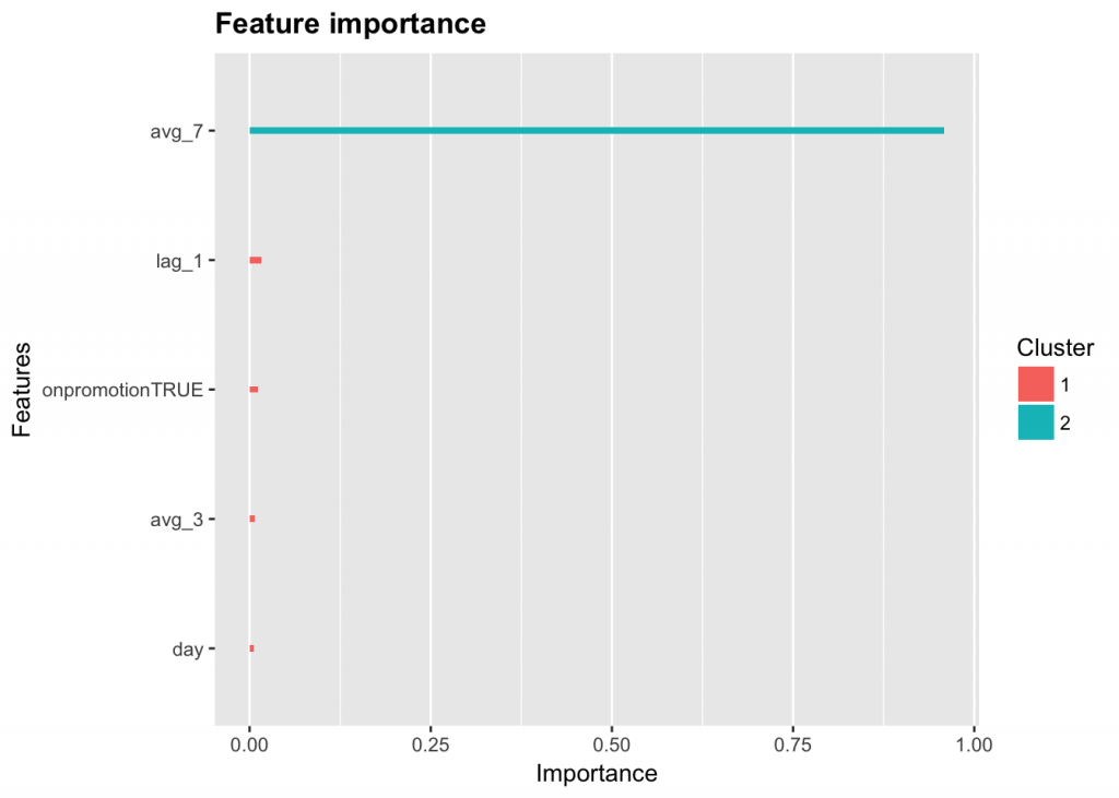
Xgb.importance shows how influential each feature was in building the model. This function helps us identify unnecessary features.
Feature Importance Plot
importance <- xgb.importance(feature_names = colnames(trainMatrix), model = model)
xgb.ggplot.importance(importance_matrix = importance)
Recursive Forecasting
One of the difficulties in this problem is we must predict sales for the next fifteen days. The current data set only has the lag and rolling mean values for the first day we must predict (2017-08-16). To predict for the entire test data set, we must recursively add the predictions to the test data set then use the updated data set to predict for the next day. One issue is that errors will propagate through the model which can decrease the accuracy of longer-term predictions.
In this for loop, we perform many of the same operations to the test data set as we did to the training data set in previous steps. If you do not understand any of the code below, look back through this post to see if that particular action was described previously.
Dates <- seq.Date(from = as.Date('2017-08-16'), by = 'day', to = as.Date('2017-08-21' ))

df_test <- df
i=1
for (i in 1:length(Dates)){

  #Order test dataset
  df_test <- df_test[order(df_test$date),]

  #Create lag variables on the testing data
  df_test <- df_test %>%
    group_by(store_nbr, item_nbr) %>%
    mutate(lag_1 = lag(unit_sales, 1)
         , avg_7 = lag(roll_meanr(unit_sales, 7), 1)
         , avg_3 = lag(roll_meanr(unit_sales, 3), 1)
         )

  #Subset testing data to predict only 1 day at a time
  test <- df_test[df_test$date == as.character(Dates[i]),]

  #Remove NAs
  test <- test[!is.na(test$avg_7),]

  #Create test matrix to build predictions
  previous_na_action<- options('na.action')
  options(na.action='na.pass')

  testMatrix <- sparse.model.matrix(~ avg_3 + avg_7 + lag_1 + day + onpromotion
                                   , data = test
                                   , contrasts.arg = c('day', 'onpromotion')
                                    , sparse = FALSE, sci = FALSE)


  options(na.action = previous_na_action$na.action)

  #Predict values for a given day
  pred <- predict(model, testMatrix)

  #Set predictions that are less than zero to zero
  pred[pred < 0] <- 0

  #Add predicted values to the data set based on ids
  df_test$unit_sales[df_test$id %in% test$id] <- pred

  # print(as.data.frame(subset(df_test, date > '2017-08-12' & date < '2017-08-23' & store_nbr == 1 & item_nbr == 103520)))
}
Here we subset the data to only include the days we predicted. We predict zero unit_sales for any NA values, convert the predictions from their log using the expm1() function and write the predictions to a csv file.
#Only include the testing dates
df_test <- df_test[df_test$date >= '2017-08-16',]

#Set NA values to zero
df_test$unit_sales[is.na(df_test$unit_sales)] <- 0

#Convert predictions back to normal unit from the log.
df_test$unit_sales <- expm1(df_test$unit_sales)

#Create solution dataset
solution <- df_test[,c('id', 'unit_sales')]

#Write solution csv
write.csv(solution, 'solution.csv', row.names = FALSE)
I hope after completing this post you are able to build your own time series forecasting models. Please comment / share if you liked this post and feel free to contact me here if you have any questions.

Contact Red Oak Strategic
.png)
Analytics
AWS Summit 2026 Reflection: From Possibility to Production Execution Last year at AWS Summit in Washington, DC, the AI conversation still ha...


Data
Introduction This is the first installment of a three-part technical series detailing the end-to-end observability and log tracking architec...


Data
The Problem: AI Pilots Are Easy to Start and Hard to Scale AI is no longer a future-state conversation for most organizations. Leadership te...
